library(stars)
library(rstac)
library(gdalcubes)
library(tmap)
library(dplyr)

gdalcubes::gdalcubes_options(parallel=24*2)California Department of Fish and Wildlife (CDFW) provides a series of data products to identify “areas of conservation emphasis” (ACE), which are currently being used as part of California’s 30x30 conservation initiative. At a recent event at the California Academy, one of the CDFW scientists mentioned it would be nice to see how the Biodiversity Intactness Index (BII) values compare to the CDFW prioritization layers. The BII (sometimes called the local or LBII) is one of a handful of indicators of global biodiversity change highlighted by GEO BON. Various attempts to estimate this indicator have been made over the past decades – the most recent and most high-resolution one currently available (and updated annually) is the Impact Observatory product based on the approach of Newbold et al and the PREDICTS database, which is available in cloud-optimized format from the Planetary Computer STAC catalog.
Aside from drowning in acronyms, this task provides a great chance to apply the same tools seen in our intro at a larger spatial scale. We will average the rasterized 100m projections from the BII over each of the 63,890 polygon tiles used in the CDFW data. Even though we are now dealing with a raster layer that involves a very derived product (BII) from a different provider (Planetary Computer), and a much larger set of polygons from a different source and in different scale and projection, the process is almost identical to the intro example.
CDFW uses a hex-based tiling scheme for their data products. Note that these pre-date the modern H3 hex tiling system, so do not provide the magic of hierarchical (zoom level) tiles. CDFW makes the ACE GIS Data freely available, but in one large zip archive. The ACE data includes may different layers all using the same hex-based tiles. The layer we pull here draws from their summary rankings on Terrestrial Irreplacability of species biodiversity.
Here I’ll use a public mirror on a Berkeley-based server for a more cloud-native access pattern so we don’t have to download the whole thing. We also index this in a simple stac catalog
url <- "/vsicurl/https://minio.carlboettiger.info/public-biodiversity/ACE_summary/ds2715.gdb"ace <- st_read(url) tm_shape(ace) + tm_polygons(fill = "RwiRankEco", col=NA)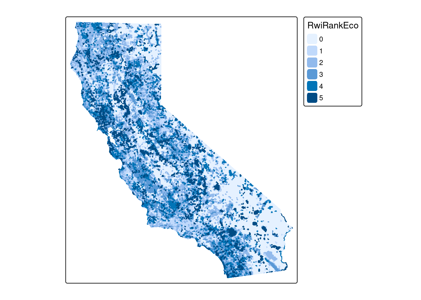
Find Biodiversity Intactness Index COG tiles from Planetary Computer using STAC search:
box <- st_bbox(st_transform(ace, 4326))
items <-
  stac("https://planetarycomputer.microsoft.com/api/stac/v1") |>
  stac_search(collections = "io-biodiversity",
              bbox = c(box),
              limit = 1000) |>
  post_request() |>
  items_sign(sign_fn = sign_planetary_computer())
Created a desired cube view
cube <- gdalcubes::stac_image_collection(items$features, asset_names = "data")
box <- st_bbox(ace)
v <- cube_view(srs = "EPSG:3310",
               extent = list(t0 = "2020-07-01", t1 = "2020-07-31",
                                left = box[1], right = box[3],
                                top = box[4], bottom = box[2]),
               dx = 100, dy=100, dt = "P1M")

Q <- raster_cube(cube,v)
Quick plot of the data at requested cube resolution.
Q |> plot(col=viridisLite::viridis(30), nbreaks=31)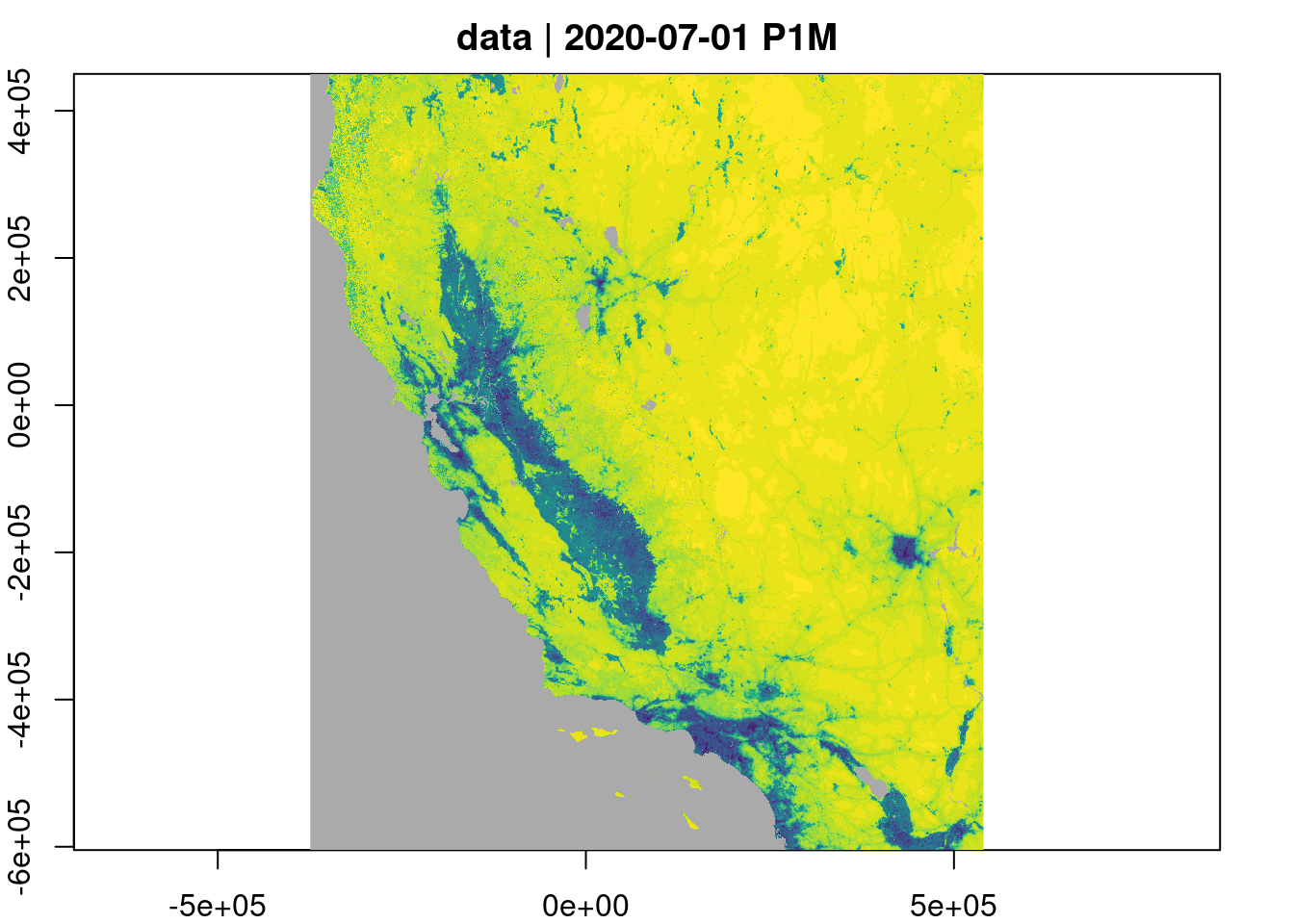
Extract mean value of the BII for each hex.
bii <- Q |> gdalcubes::extract_geom(ace, FUN=mean)Plots
View the average BII index values by ACE hexagon:
tmap_mode("plot")

# color palette
viridis <- tm_scale_continuous(values = viridisLite::viridis(30))

bii <- ace |>
  tibble::rowid_to_column("FID") |>
  left_join(bii)

tm_shape(bii) +
  tm_polygons(fill = "data", col=NA, fill.scale = viridis)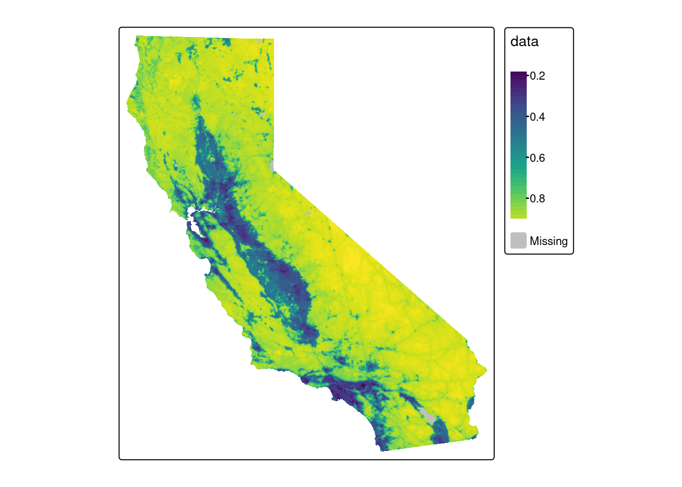
Let’s zoom in manually:
tmap_mode("plot")
sf = st_bbox(c(xmin=-123, ymin=38.5, xmax=-122, ymax=37.5), crs=4326)
tm_shape(bii, bbox = sf) +
  tm_polygons(fill = "data", col=NA,
              fill.scale = viridis)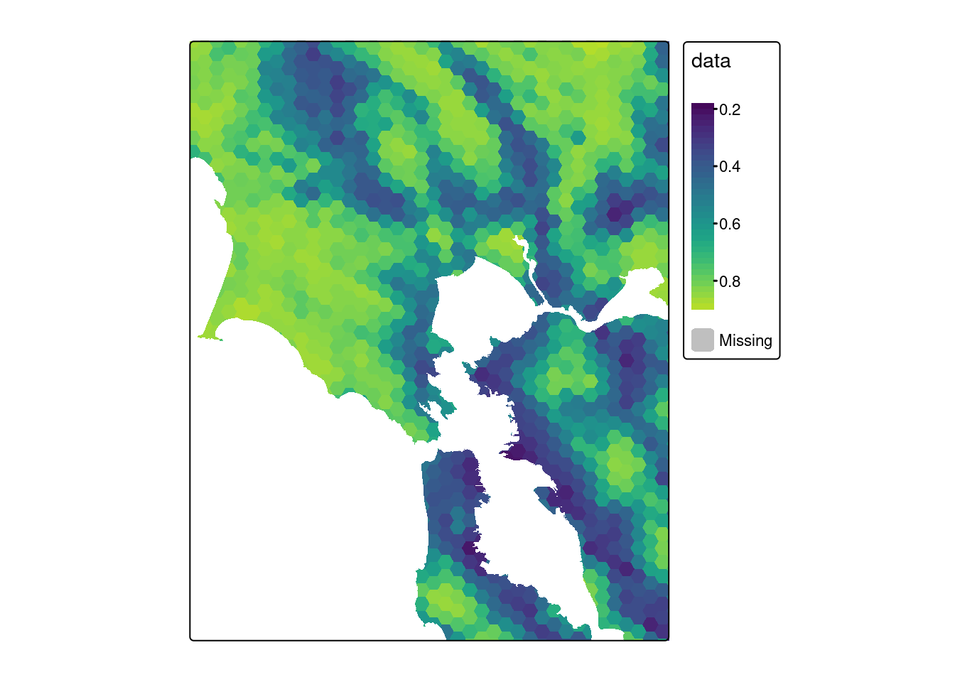
Now that we have the data in convenient and familiar data structures, it is easy to analyze. On average, a hexagon’s irreplacability rank shows little correlation with BII:
library(tidyverse)
bii |> as_tibble() |> select(-Shape) |>
  group_by(RwiRankEco) |>
  summarise(BII = mean(data, na.rm=TRUE),
            sd = sd(data, na.rm=TRUE)) |>
  ggplot(aes(RwiRankEco, BII)) +
  geom_col(aes(fill=RwiRankEco)) +
  geom_linerange(aes(ymin = BII-2*sd, ymax = BII+2*sd), col = "grey50")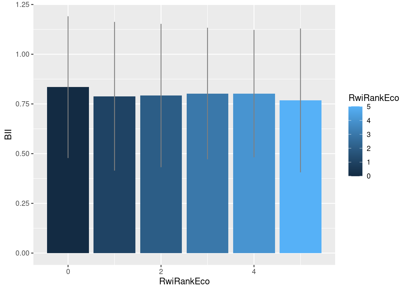
Leaflet map
We can also render an interactive leaflet plot where we can zoom in and out and toggle basemaps:
tmap_mode("view")
bii <- Q |> st_as_stars()
map <-
  tm_shape(bii) +
  tm_raster(col.scale = viridis) +
  tm_shape(ace) +
  tm_polygons(fill = "RwiRankEco", col=NA)

tmap_save(map, "bii_hexes.html")